PSpice Examples for EE-201
Hadi Saadat
DC NODE-VOLTGE AND MESH CURRENT ANALYSIS
To obtain current and voltage in a DC circuit, the analysis is performed with the simple Load Bias Point.
If any AC sources are present in the circuit, those sources are set to zero. All capacitors are replaced by the pen-circuit, and all inductors are replaced by short circuits. From the Analysis menu, choose Setup. The Analysis setup dialog box appears. Click the Enabled check box in the Bias Load Point option. To monitor a DC node voltage a VIEWPOINT is placed at that node. To obtain the DC current in a branch an IPROBE is placed in that branch. The reference direction of current for the circuit elements is from the first listed subscript to the second one. You may have to rotate the IPROBE from the Edit Menu (or use Ctrl R), so that the reading is in the assumed direction of current. To see the IPROBE direction of current, from the Analysis menu open the Examine Netlist file and check the order of element nodes.
Bias voltages and currents Display
From the Analysis menu you can customize the Display results on Schematics to show selected DC voltages and currents. You can enable or disable the bias voltages and currents by using the toolbar buttons
V and
I. (You may use display results in place of Viewpoint and Iprobe).
 Download PSPICE Schematics files for EE-201 Examples. To view the Pspice examples you need to download the OrCAD Viewer Free Download. To run the examples, students can download the complete Free OrCAD Software for Students.
Example 1 (EE201ex1.sch)
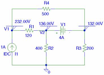
Use the PSpice Schematics to construct the circuit below and obtain the node voltages.
To obtain the node voltages a VIEWPOINT is placed at each node labeled V1, V2, and V3 (To assign a name or a number to a node double click on that node).
Schematics Netlist
R_R3 $N_0001 0 200
R_R4 V1 $N_0001 500
R_R2 V2 0 400
V_V1 V2 $N_0001 4A
R_R1 V1 V2 120
I_I1 0 V1 DC 1A
Top of Page
Example 2 (EE201ex1.sch)
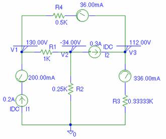
Use the PSpice Schematics to construct the circuit below and obtain the node voltages and mesh currents. Assume a clockwise direction for the mesh current To obtain the node voltages a VIEWPOINT is placed at each node labeled V1, V2, and V3 (To assign a name or a number to a node double click on that node).
To obtain the three mesh currents an IPROBE is placed in each mesh. Note that each IPROBE is rotated (Ctrl R) in such a way as to obtain the mesh current for the assumed clockwise direction.
Schematics Netlist
R_R1 V1 V2 1K
R_R4 V1 $N_0001 0.5K
R_R3 $N_0002 0 0.33333K
R_R2 V2 0 0.25K
I_I1 0 $N_0003 DC 0.2A
I_I2 V2 V3 DC 0.3A
v_V2 $N_0001 V3 0
v_V3 V3 $N_0002 0
v_V1 $N_0003 V1 0
Top of Page
Example 3 (EE201ex3.sch)
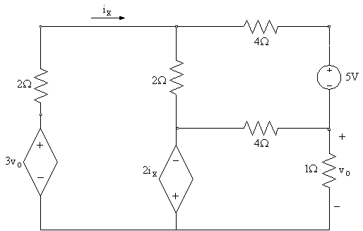
Determine the node voltages for the circuit containing a Voltage-Controlled Voltage Source as shown.
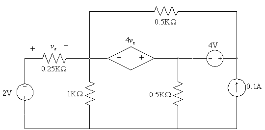
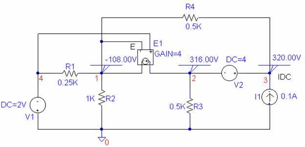
Schematics Netlist
R_R3 2 0 0.5K
R_R1 4 1 0.25K
V_V2 3 2 DC 4
E_E1 2 1 4 1 4
R_R2 1 0 1K
I_I1 0 3 DC 0.1A
V_V1 0 4 DC 2V
R_R4 1 3 0.5K
Top of Page
Example 4 (EE201ex4, sch)
The circuit below contains a Voltage-Controlled Voltage Source and a Current-Controlled Voltage Source. Determine the node voltages and the controlled current of the dependent source.
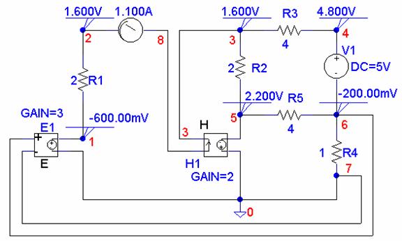
* Schematics Netlist *
R_R5 5 6 4
R_R4 6 0 1
R_R3 3 4 4
R_R2 3 5 2
R_R1 2 1 2
V_V1 4 6 DC 5V
E_E1 1 0 6 0 3
H_H1 0 5 VH_H1 2
VH_H1 8 3 0V
v_V2 2 8 0
Top of Page
Example 5 (EE201ex5.sch)
- Find the current in the 3.5 W resistor in the circuit (a).
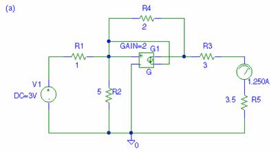
(b) Obtain the Thevenin's equivalent circuit with respect to the terminal of the 3.5W resistor.
With the 3.5W resistor removed, we find the open-circuit voltage, and with load resistance shorted we find the short-circuit current. Then, the Thevenin's impedance is
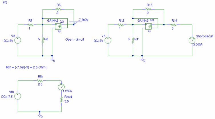
Schematics Netlist
V_V1 $N_0001 0 DC 3V
R_R2 $N_0002 0 5
R_R1 $N_0001 $N_0002 1
G_G1 $N_0003 $N_0002 $N_0002 0 2
R_R4 $N_0002 $N_0003 2
R_R3 $N_0003 $N_0004 3
V_V3 $N_0005 0 DC 3V
R_R6 $N_0006 0 5
R_R7 $N_0005 $N_0006 1
R_R8 $N_0006 $N_0007 2
G_G2 $N_0007 $N_0006 $N_0006 0 2
R_R12 $N_0009 $N_0008 1
R_R13 $N_0008 $N_0010 2
V_V5 $N_0009 0 DC 3V
R_R11 $N_0008 0 5
R_R14 $N_0010 $N_0011 3
G_G3 $N_0010 $N_0008 $N_0008 0 2
R_Rth $N_0013 $N_0012 2.5
V_Vth $N_0013 0 DC -7.5
R_Rload $N_0014 0 3.5
R_R5 $N_0015 0 3.5
v_V2 $N_0004 $N_0015 0
v_V7 $N_0011 0 0
v_V9 $N_0012 $N_0014 0
2. Transfer function
Computes the gain and the input and output resistances and automatically sends the results to the output file. To specify the transfer function, choose Setup from the Analysis menu and open the Transfer Function dialog box. In the Output Variable box specify the output voltage, and in the Input Source box type the input source name. The transfer function analysis can be used conveniently to obtain the Thevenin's equivalent circuit. The use of this analysis to obtain the Thevenin's equivalent circuit is demonstrated in the following example
Top of Page
Example 6 (EE201ex6.sch)
Use the transfer function analysis to obtain the Thevenin's equivalent circuit for the circuit of Example 5.
We want to obtain the Thevenin's equivalent circuit with respect to the 3.5 W resistor. The 3.5 W resistor is replaced by an open circuit. Since in PSpice two or more elements must be connected to each node, the 3.5 W resistor is replaced by an infinitely high value resistor as shown. A VIEWPOINT is added at node 4 to display the open-circuit voltage (Thevenin's voltage). To obtain the output or Thevenin's resistance, the transfer Function is enabled. In the Output variable box we type V(4), and in the Input Source box, we type V1.
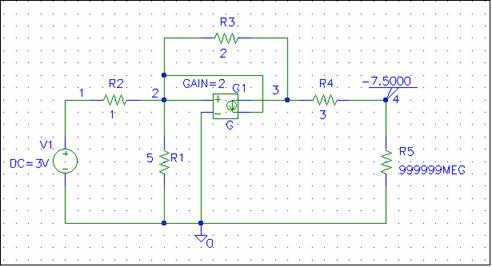
Schematics Netlist
V_V1 1 0 DC 3V
R_R1 2 0 5
R_R2 1 2 1
G_G1 3 2 2 0 2
R_R3 2 3 2
R_R4 3 4 3
R_R5 4 0 999999MEG
In addition to the DC analysis result, the output file contains the Transfer Function analysis results as follows
SMALL-SIGNAL CHARACTERISTICS
V(4,0)/V_V1 = -2.500E+00
INPUT RESISTANCE AT V_V1 = 6.000E+00
OUTPUT RESISTANCE AT V(4,0) = 2.500E+00
Thus, the Thevenin's voltage is V4 = -7.5 V, and the Thevenin's resistance is the output resistance 2.5 W.
2. DC Sweep
DC voltage or current sources may be swept over a range through the use of the DC Sweep Analysis. The DC Sweep is similar to the node voltage analysis, but adds more flexibility. In the DC sweep, the input variable is varied over a range of values. For each value of the input variable, the DC operating point is computed. If the transfer function is also enabled the small-signal DC gain and the input/output resistances are also computed.
Top of Page
Example 7 (EE201ex7.sch)
For the circuit shown print and plot the voltage V23, IR2, and IR3 as the input voltage is varied from 0 to 100 V in 5 V increment. Select the Setup from the analysis menu, click the DC Sweep dialog button. The DC Sweep dialog box appears. For the Sweep Variable type select the voltage source, and set its name to V1. Using the Sweep type linear, specify the starting value, end value and increment. IPRINT and VPRINT2 are inserted in the appropriate locations to send the desired currents and voltages to the output file. To include the DC values double click on each print icon and set the DC = to yes.
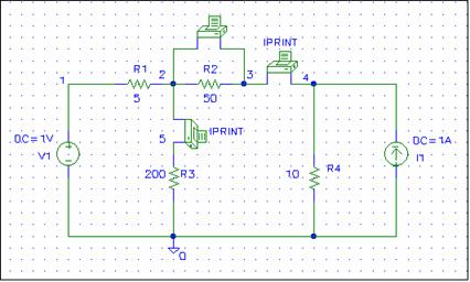
The Probe result which includes traces V (2,3) I (R2), and I (R3) is shown below.
The desired currents and voltage copied from the output file are tabulated below.
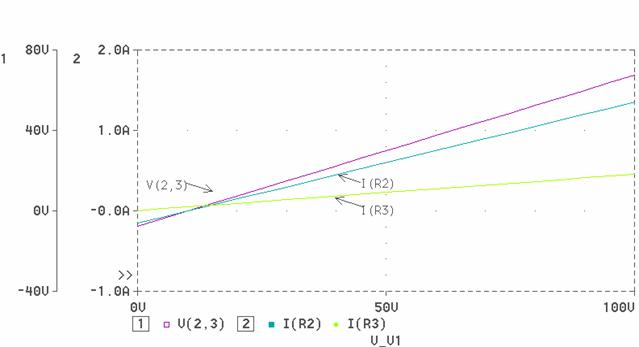
V_V1 V(2,3)
0.000E+00 -7.707E+00
5.000E+00 -3.947E+00
1.000E+01 -1.880E-01
1.500E+01 3.571E+00
2.000E+01 7.331E+00
2.500E+01 1.109E+01
3.000E+01 1.485E+01
3.500E+01 1.861E+01
4.000E+01 2.237E+01
4.500E+01 2.613E+01
5.000E+01 2.989E+01
5.500E+01 3.365E+01
6.000E+01 3.741E+01
6.500E+01 4.117E+01
7.000E+01 4.492E+01
7.500E+01 4.868E+01
8.000E+01 5.244E+01
8.500E+01 5.620E+01
9.000E+01 5.996E+01
9.500E+01 6.372E+01
1.000E+02 6.748E+01
V_V1 I(V_PRINT3)
0.000E+00 -1.541E-01
5.000E+00 -7.895E-02
1.000E+01 -3.759E-03
1.500E+01 7.143E-02
2.000E+01 1.466E-01
2.500E+01 2.218E-01
3.000E+01 2.970E-01
3.500E+01 3.722E-01
4.000E+01 4.474E-01
4.500E+01 5.226E-01
5.000E+01 5.977E-01
5.500E+01 6.729E-01
6.000E+01 7.481E-01
6.500E+01 8.233E-01
7.000E+01 8.985E-01
7.500E+01 9.737E-01
8.000E+01 1.049E+00
8.500E+01 1.124E+00
9.000E+01 1.199E+00
9.500E+01 1.274E+00
1.000E+02 1.350E+00
V_V1 I(V_PRINT1)
0.000E+00 3.759E-03
5.000E+00 2.632E-02
1.000E+01 4.887E-02
1.500E+01 7.143E-02
2.000E+01 9.399E-02
2.500E+01 1.165E-01
3.000E+01 1.391E-01
3.500E+01 1.617E-01
4.000E+01 1.842E-01
4.500E+01 2.068E-01
5.000E+01 2.293E-01
5.500E+01 2.519E-01
6.000E+01 2.744E-01
6.500E+01 2.970E-01
7.000E+01 3.195E-01
7.500E+01 3.421E-01
8.000E+01 3.647E-01
8.500E+01 3.872E-01
9.000E+01 4.098E-01
9.500E+01 4.323E-01
1.000E+02 4.549E-01
Top of Page
Example 8 (EE201ex8.sch)
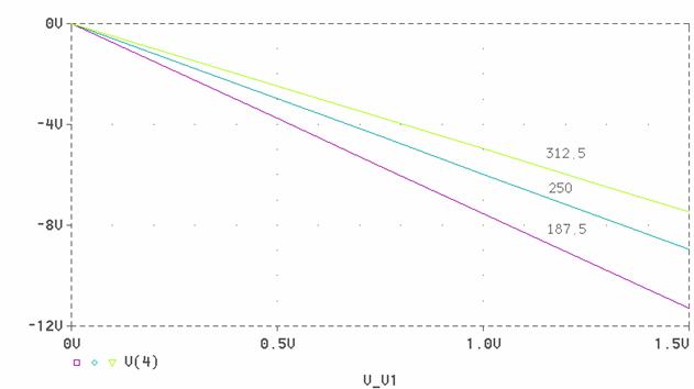
The circuit shown below represents an amplifier circuit modeled by a current-controlled current source. The input voltage is varied from 0 to 1.5 V with an increment of 0.25 V. The resistance Re changes by ± 25%. Plot the DC transfer characteristic output voltage V4 versus the input voltageV1 for each value of the resistance Re.
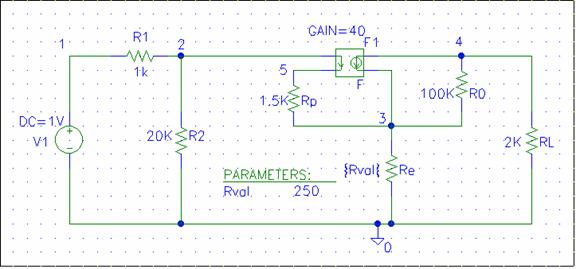
Select the Setup from the analysis menu, click the DC Sweep dialog button. The DC Sweep dialog box appears. For the Sweep Variable type select the voltage source, and set its name to V1. Using the Sweep type linear, specify the starting value, end value and increment (0, 0.25, and 1.5).
The Parametric Sweep can be used to change the value of the resistor Re. To do this, get a part called PARAM from Special.slb and place it in your circuit. Double click on the text PARAMETERS. The attributes allow you to define up to three different variable parameters. For NAME1= define a parameter,
say Rval, and for VALUE1= set an initial value of 250. Click the OK button to accept the attribute. We must now change the value of Re to the name of the parameter. Double click on the value of R1 and in place of its value type in the text {Rval}. Next select the Analysis and then Setup and click the Parametric button. Mark Global Parameter, set Name to Rval. Under Sweep Type, mark Value List and set the Values: to 187.5 250 312.5. Perform the simulation.
The probe result is as shown.
AC Analysis
This is used for the following analysis:
- Steady-state analysis: Finding the steady-state phasor voltages and currents at a single frequency
- Frequency response: Finding the frequency response of a circuit over a range of frequencies.
To run an AC Analysis, we require an AC source with AC specifications such VSRC, ISRC or VAC and IAC. In the Analysis setup dialog box, click on the AC sweep button. Complete the AC Sweep and Noise Analysis box as required. For AC analysis at a single frequency say 60 Hz, select Linear AC Sweep, set Total Pts: to 1, Start Freq: to 60, and End freq: to 60. For frequency response over a wide range of frequencies you can sweep the following type
Linear Specifies a linear variation.
Octave Specifies an octal variation
Decade Specifies a decade variation (Logarithmic scale)
The following parts called Printpoints are available for writing the simulation results to the output files:
VPRINT1 VPRINT2 IPRINT VPLOT1 VPLOT2
In all of the above Printpoints , you can specify one or more analysis type. To do this double click on the symbol, double click on the analysis type for example AC, and set its value text box to any non-blank value, such as Yes or 1. If AC is set, then one or more output format may also be set: MAG(magnitude), PHASE, REAL, IMAG(imaginary), or dB(decibels).
For multiple frequencies, the results can be viewed graphically using Probe to generates plots of magnitude versus frequency, or plots of phase versus frequency. To plot the magnitude of a signal in probe, specify V(expression) or I(expression). To plot the phase angle of a signal, specify VP(expression). Use the command dB(expression) to plot a trace in decibels. Alternatively, you can use special markers to mark one or more variables to be automatically plotted in the Probe. In the Schematic Window, select Markers, Mark Advanced, choose the desired markers from the following, OK, place the marker at the desired location.
vdb vphase vreal vimaginary
idb iphase ireal iimaginary
Top of Page
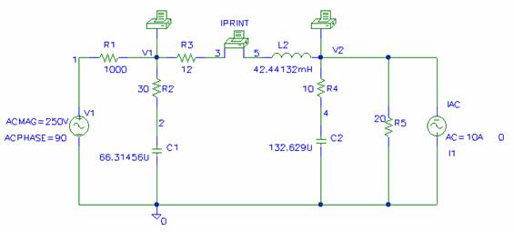
Example 9 EE201ex9.sch
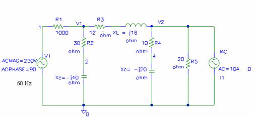
(a) Use node-voltage analysis to find the magnitude and phase angle of the node voltages V1 and V2, then find magnitude and phase angle of current in R3.

Transforming the voltage source to the current source and writing the node-voltage equation results in

or
Current in R3 is

(b) (EE201ex9.sch) The voltage source and the current source frequency are 60 Hz. Use PSpice and AC Analysis for a single point 60 Hz to obtain the node voltages V1 and V2, and current in R3. Use VPRINT, and IPRINT to send the node voltages and current to the output file. In the VPRINT and IPRINT dialog box set the attributes AC, MAG, and PHASE to yes.
The following results are extracted from the Output File
FREQ VM(V1) VP(V1)
6.000E+01 9.605E+01 -5.134E+01
FREQ VM(V2) VP(V2)
6.000E+01 9.953E+01 -2.785E+01
FREQ IM(V_PRINT4) IP(V_PRINT4)
6.000E+01 1.998E+00 1.724E+02
Top of Page
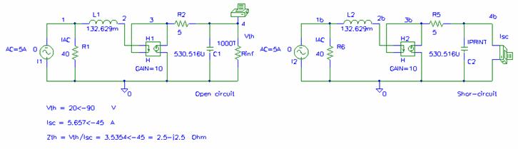
Example 10 (EE201ex10.sch)
In the circuit shown find the Thevenin's equivalent circuit with respect to terminals ab.
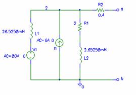
In order to obtain the Thevenin's voltage, a high resistance, Rinf is connected across terminal ab. VPRINT1 is used to send the voltage magnitude and phase angle to the Output File. The AC, MAG, and PHASE attributes are set to yes. To find the Thevenin's impedance, terminal ab is shorted through an IPRINT device used as an ammeter. The AC, MAG, and PHASE attributes of OPRINT are set to yes.
From the Output File,


Top of Page
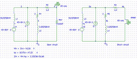
Example 11 (ee201ex11)
In the following circuits a single point 60 Hz AC Analysis is set up for an open circuit and a short-circuit conditions to obtain the Thevenin's equivalent circuit. VPRINT1 and an IPRINT are used to include Vth and Isc in the output file. The AC, MAG, and PHASE attributes of VPRINT1 and IPRINT are set to yes.
From the Output File,


Top of Page
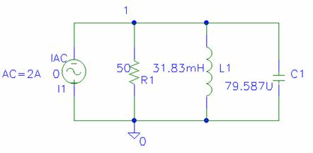
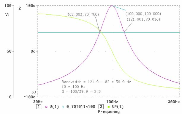
Example 12 (ee201ex12)
For the parallel RLC circuit shown, use PSpice and Probe to plot voltage magnitude and phase angle over a range of 30 to 300 Hz in increment of 1 Hz (Total point =271). Determine the resonant frequency. Also draw the 0.707 V0(max) line and estimate the circuit bandwidth and the Q-factor.
Top of Page
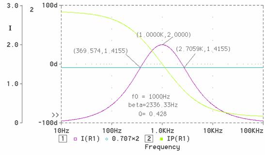
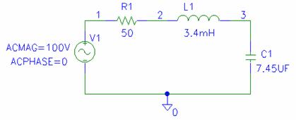
Example 13 (ee201ex13)
For the series RLC circuit shown, use PSpice, and AC Analysis to sweep the frequency from 10Hz to 100KHz over a decade variation with 200 points per decade.
(a) Use Probe to plot the current magnitude and phase angle. Determine the resonant frequency. Also draw the 0.707( V0(max)) line and estimate the circuit bandwidth b, and the Q-factor.

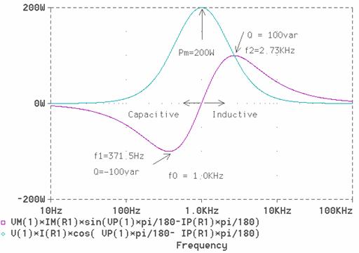
(b) On a separate graph plot the real and reactive power delivered to the circuit as a function of frequency.

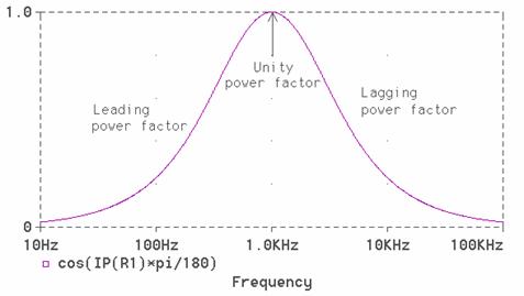
(c) On a separate graph, plot the power factor as a function of frequency.

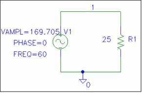
Example 15 a (ee201ex15a)
(i) Determine the real power in the circuit shown.
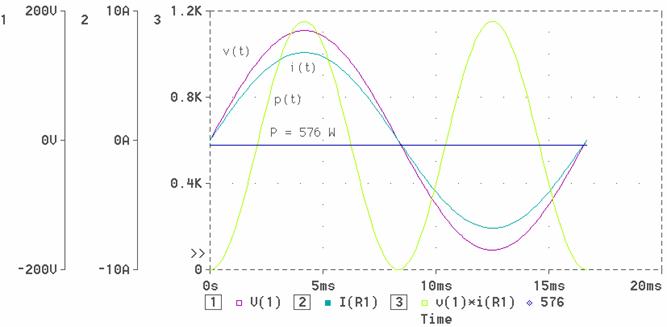
(ii) Use PSpice and Transient Analysis to obtain a plot of the instantaneous voltage v1(t), i(t), and the instantaneous power p(t).


(i)

(ii) The Final Time in the Transient Analysis is set to T = 1/60 = 16.667ms. The following instantaneous quantities and the average power are plotted.
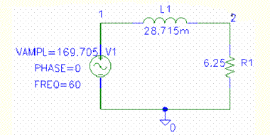
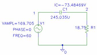
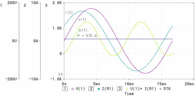
Example 15 b (ee201ex15b)
(i) Determine the real power in the circuit shown.
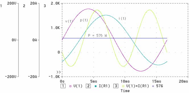
(ii) Use PSpice and Transient Analysis to obtain a plot of the instantaneous voltage v1(t), i(t), and the instantaneous power p(t).


(ii) The Final Time in the Transient Analysis is set to T = 1/60 = 16.667ms. The following instantaneous quantities and the average power are plotted
Top of Page
Example 15 c (ee201ex15c)
(i) Determine the real power in the circuit shown.

(ii) Use PSpice and Transient Analysis to obtain a plot of the instantaneous voltage v1(t), i(t), and the instantaneous power p(t).


(ii) The Final Time in the Transient Analysis is set to T = 1/60 = 16.667ms. The following instantaneous quantities and the average power are plotted
Top of Page